Pacing Strategy for Running Around the Bay

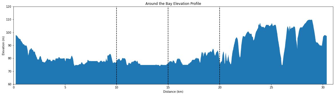
A friend was wondering how to pace themselves at the Around the Bay 30km road race on March 27th. The race has a unique elevation profile, with several significant hills in the last 10km.

For a runner hoping to meet a specific time it begs the question of whether they should start the race faster than their goal race pace or not. A faster starting pace in anticipation for slowing down on the hills near the end of the race makes sense, but begs the question of how much faster? Conventional running wisdom is to run “even splits”, which is running the same pace for the entirety of a race. As I’m also going to be running the race this year, I want to know what the optimal pacing strategy for the Around the Bay course is. I’ll do that by comparing how well popular heuristics and models align with historical results at Around the Bay. First let’s review the methods that will be compared.

Pacing Heuristics

Even Pace/Even Effort

The simplest of the pacing strategies are even pace, and even effort. Even pacing simple means to run the same pace throughout the race. It’s a good strategy for a flat course, but can be near impossible to replicate on a hilly course. The alternative is even effort, where an exertion level is kept constant, as pace is slowed on uphills and increased on downhills. This is a good simple heuristic, but can be difficult to follow in a race. Unless one is diligently heart rate or power training, it’s difficult to start and maintain an effort throughout a race. Thankfully, there are some guidelines for running at even effort.

First there are the rules developed from two of the most infamous studies on the subject.

Jack Daniels

+12-15s/mile/% gradient incline

-8s/mile/% gradient decline

The legendary coach Jack Daniels is heavily quoted for a comment he (jtupper) made online referencing a study performed on the subject. The post suggested that 12 to 15 seconds should be added per mile per increase in gradient percent. The study also suggested that a downhill subtracts 8 seconds per mile per decline in gradient percent.

John Kellogg

+9.2s/mile/% gradient incline

John Kellogg made similar online posts, which have been summarized in this document. His number was a more conservative 9.2 seconds should be added per mile per increase in gradient percent, which he further generalized to 1.74s for each 10ft elevation gain regardless of distance covered. John never specified the effect of the downhills so we won’t use his numbers in our analysis.

Jack and John both expressed that there formulas are merely guidelines, that seemed accurate on average for the people they studied. Since the studies were on runners of relatively similar ability to myself they should have some good information for me. Their guidelines don’t scale with pace, so they won’t be as accurate for runners much slower than 4min/km. For a more general tool we need a model.

Models

Grade Adjusted Pace

Strava has a model they apply for all subscribers on their platform called Grade Adjusted Pace. I’ll discuss it further in an upcoming post about cross country courses. This blog post details the model and compares it with a study from a 2002 paper on the matter. For our comparison we will use both the Strava and Minetti curves. As shown in the diagram, they use Equal Energy Cost and Equal Heartrate as a proxies for even effort.

Normalized Graded Pace

TrainingPeaks has a similar metric called Normalized Graded Pace, but there is less information on how it is calculated so I won’t be investigating it here.

Data Mining

Results

Most of the data for this analysis is scraped from results posted on https://www.sportstats.ca/. For the races from 2016-2019 the 10km, 15km, 20km, and finish splits for each athlete are available. Splits from earlier years are accessible, but more difficult to obtain, and the 4 years captured have shown to be sufficient for our purposes.

GPS

To get the course elevation profile I’ve used the gps recordings from my own previous runs on the course. The gps files are parsed into a pandas dataframe for easy calculations and plotting.

Data Exploration

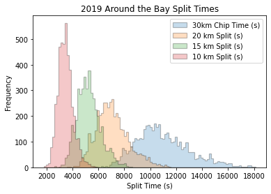
The results for the four years from 2016-19 were all combined for analysis. The split time distributions show the predictable widening of the distribution as the race spreads out over time, and a small deviation from normal as athletes who went out too fast cause a long tail to the final distributions.

The raw data only has the running time for each athlete at each distance (10km, 15km, 20km, 30km), but we want to look at the pace they ran for each of the segments (0-10km, 10-15km, 15-20km, 20-30km). Calculating these gives us these averages.

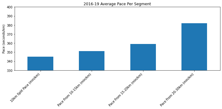
As we expected, the final 10km of the race are slowest (largest pace). On average the first 10km is 40s/km faster than the last. A slow finish is fairly common for most road races as most runners are optimistic with their pacing strategy. Since I am going to plan for success, I’ll have to remove some of these outliers.

Data Filtering

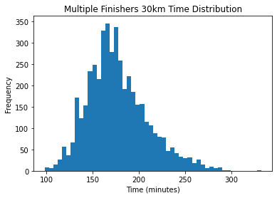
Keeping my filtering as simple as possible I’ve selected two comparison criteria. The first is to only look at runners that have previously run the race in my dataset. The thought is that these multiple finishers will know the course well and how they should pace themselves. Dropping each runner’s first performance in the dataset leaves in a wide distribution of times and keeps 4622 performances (26% of the 17440 in the dataset).

The other more relevant filter is to keep only the “elite” athletes who ran faster than two hours. Though the definition of elite is up for debate, this is the top 1.6% of all finishers, and leaves just 279 performances. This is large enough for me to feel confident in the aggregated results while maximizing the amount of runners that ran close to an optimal pacing strategy. My assumption is that on average elite runners maintain an even effort.

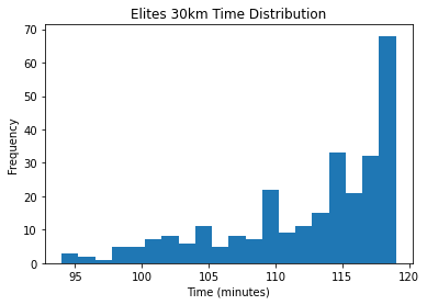
Being the leading end of the distribution, most of the times are near the two hour mark.

Model Evaluation

Race Result Analysis

With these filters in place we can take each runners pace for each segment and divide that by the average pace for the entire race to get a percentage.

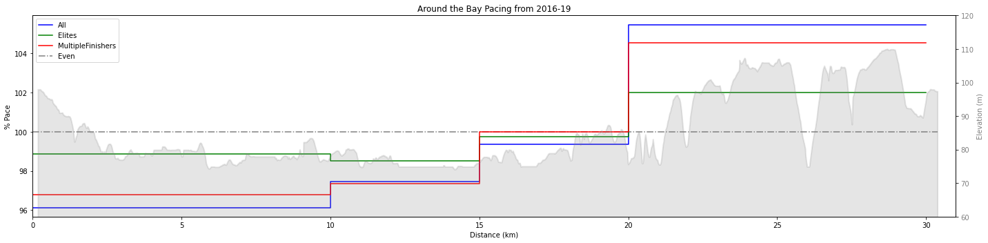
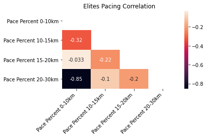
The different filters are plotted along the course profile and compared with the even pace heuristic (constant 100% pace). Each group ran faster (pace <100%) for the first 20km of the race, and slower for the last 10km. This feels right since the first two-thirds of the race are downhill or flat, and the last third is very hilly. All the runners combined highlights the suboptimal pacing of the average Around the Bay runner as they tend to go out significantly faster than they finish. On average the runners don’t save enough energy for the hills at the end of the race. To back this up, if we look at the correlation between the paces, we can see that best determinant for a runner’s pace in the last 10km of the race is what they ran in the first 10km.

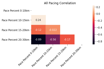
A correlation of -0.89 is very strong, and means that on average the athletes that start too fast finish the slowest.

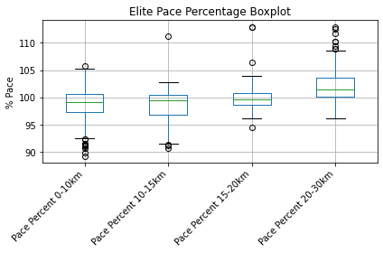
The multi-finishers tend to run closer to even splits, while the elite runners only have 3% variation in pace. However, the elite filter is not perfect, as there is are several outliers that seem to start out too fast (10% faster than they average!). This shifts our averages slightly to faster starts and slower finishes, but not significantly so we’ll leave them in.

All of this is informative, but hasn’t completely answered the question about what pacing strategy is optimal. I want to trust the average elite pacing, but it could be that the outliers are racing optimally. In an attempt to validate their performance we’ll include the other pacing models.

Grade Adjusted Pace Model

To include the Grade Adjusted Pace models I calculated the gradient throughout the course and applied each model. I then averaged the percentage pace over each segment.

To use the Jack Daniels equation I converted the time change in each segment to a percentage by comparing against my goal pace (3:36min/km). With slower goal paces the predicted effect by this formula lessens as it suggests adding a constant time to all performances, so seen as a percent it would regress toward even pacing.

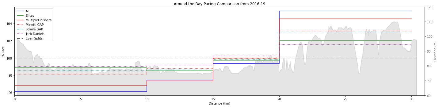
Interestingly, the closest model to the elite performance was actually the Jack Daniels formula. I think this is because the Jack Daniels study was done on elite athletes, while the Strava and Minetti studies were more for the average runner. With this comparison it does validate to me that the elite athletes have followed a good pacing strategy, as they are within 1% of each pacing model.

Prescription

The simplified takeaway from this is that runners at Around the Bay should average the first half of the race at around 1% faster than their goal pace. This sets them up to run an even effort for the duration of the race, providing some banked time to lose in the hills. For me that means starting two to three seconds per kilometer faster than my goal pace. Speaking from experience, the last 10 kilometers is no longer about holding yourself back with proper pacing. Instead you are pushing yourself to the limit as you fight towards the finish line. Slowing down on this section is to be expected, and maintaining a pace 2-3% slower than goal pace in this section is something to be extremely happy with.